Introduction
Past research and the application scope of the current research project point to several considerations relevant to the evaluation of alternative accessibility measures for transportation planning.
These considerations include: (a) the theoretical basis of the measure; (b) the ease of aggregation over time, space, activity, mode and individual or household type; (c) the data needed for estimation; and (d) application and performance of the accessibility measure.
The focus of this report is on assessing alternative accessibility measures: place-based (gravity type, cumulative opportunity) and individual-based (time-space, logsum).
Accessibility Measures
1. Place-Based Access
1.1 Gravity Type
(i) Inverse Power Model
where $\alpha = 0.8$, $W_j$ is the weighted area of location j and $d_{ij}$ is the travel time in minutes between location $i$ and $j$.
Reference: Bhat, M., Handy, S., Kockelman, K., and Mahmassani, H. “Assessment of Accessibility Measure.” Center for transportation research. University of Texas at Austin.
(ii) Exponential Model
where $\beta = 0.12$
Reference: Bhat, M., Handy, S., Kockelman, K., and Mahmassani, H. “Assessment of Accessibility Measure.” Center for transportation research. University of Texas at Austin.
(iii) Gaussian Model
where $v = 10$
Reference: Bhat, M., Handy, S., Kockelman, K., and Mahmassani, H. “Assessment of Accessibility Measure.” Center for transportation research. University of Texas at Austin.
1.2 Cumulative Opportunity
(i) Rectangular
where $f(d_{ij})$ = 1 for $d_{ij}\leqslant T (T = 30) $, 0 otherwise.
Reference: Bhat, M., Handy, S., Kockelman, K., and Mahmassani, H. “Assessment of Accessibility Measure.” Center for transportation research. University of Texas at Austin.
(ii) Negative Linear
where $f(d_{ij}) = 1-\dfrac{t}{T}$ for $d_{ij}\leqslant T (T = 30) $, 0 otherwise.
Reference: Bhat, M., Handy, S., Kockelman, K., and Mahmassani, H. “Assessment of Accessibility Measure.” Center for transportation research. University of Texas at Austin.
2.Individual-Based Access
2.1 Time-Space
(i) Potential Path Space (PPS) and Weighted Sum of Opportunity ($A_s$):
where $t_i$ is the last ending time of the activity at location $i$, $t_j$ is the earliest starting time of the activity at location $j$ and $v$ is the average travel speed on the transportation network
where $I(k) = 1$ if $k$ is within the feasible opportunity set, 0 otherwise.
Suppose the case that there are 100 activities happening in the area and each person performs 5 activities with random position, starting time and ending time.
The first step is to calculate for each activity whether it is within the range of potential path space (PPS). The next step is to sum up all the activities that are reachable by the PPS.
Reference: Kwan, M. “Space-time and Integral Measure of Individual Accessibility: A Comparative Analysis Using a Point-based Framework.” Geographical Analysis, Vol. 30, No. 3 (July, 1998) Ohio State University Press
2.2 LogSum
(i) LogSum Exponential:
The values calculated and reported here are the log sum of distances, not accessibility measure.
Reference: Kwan, M. “Space-time and Integral Measure of Individual Accessibility: A Comparative Analysis Using a Point-based Framework.” Geographical Analysis, Vol. 30, No. 3 (July, 1998) Ohio State University Press
Model Description
To investigate the influence of location, density, skill-level location, and transportation on accessibility, we set up a model with varying inputs to be specified. The general inputs to the model is the number of people, the number of jobs, city size, city center size, and city scale (large city or small city). The accessibility measures we use are negative linear cumulative opportunity measure and exponential gravity-type measure.
Model Parameters
Basic setup:
1000 people, 1000 households, 100 zones, 800 jobs
Quality:
Set as a constant 1 for walking, 2 for bus and 3 for driving
HH(Household Position):
Various assignments according to cases (random to get (x,y) position in the whole region and group skill level together)
Work status:
Random assign work status to each person
Job Density:
Concentrated in the center/outer/mixed of the city with skill level grouping together according to city scale
Control Variable Comparison
The control variable (or scientific constant) in scientific experimentation is the experimental element which is constant and unchanged throughout the course of the investigation. The control variable strongly influences experimental results, and it is held constant during the experiment in order to test the relative relationship of the dependent and independent variables. The control variable itself is not of primary interest to the experimenter.
In transportation accessibility measure, four variables (household location relative to job location, job density, skill level distribution, transportation method change) are controlled to explore their respective influence.
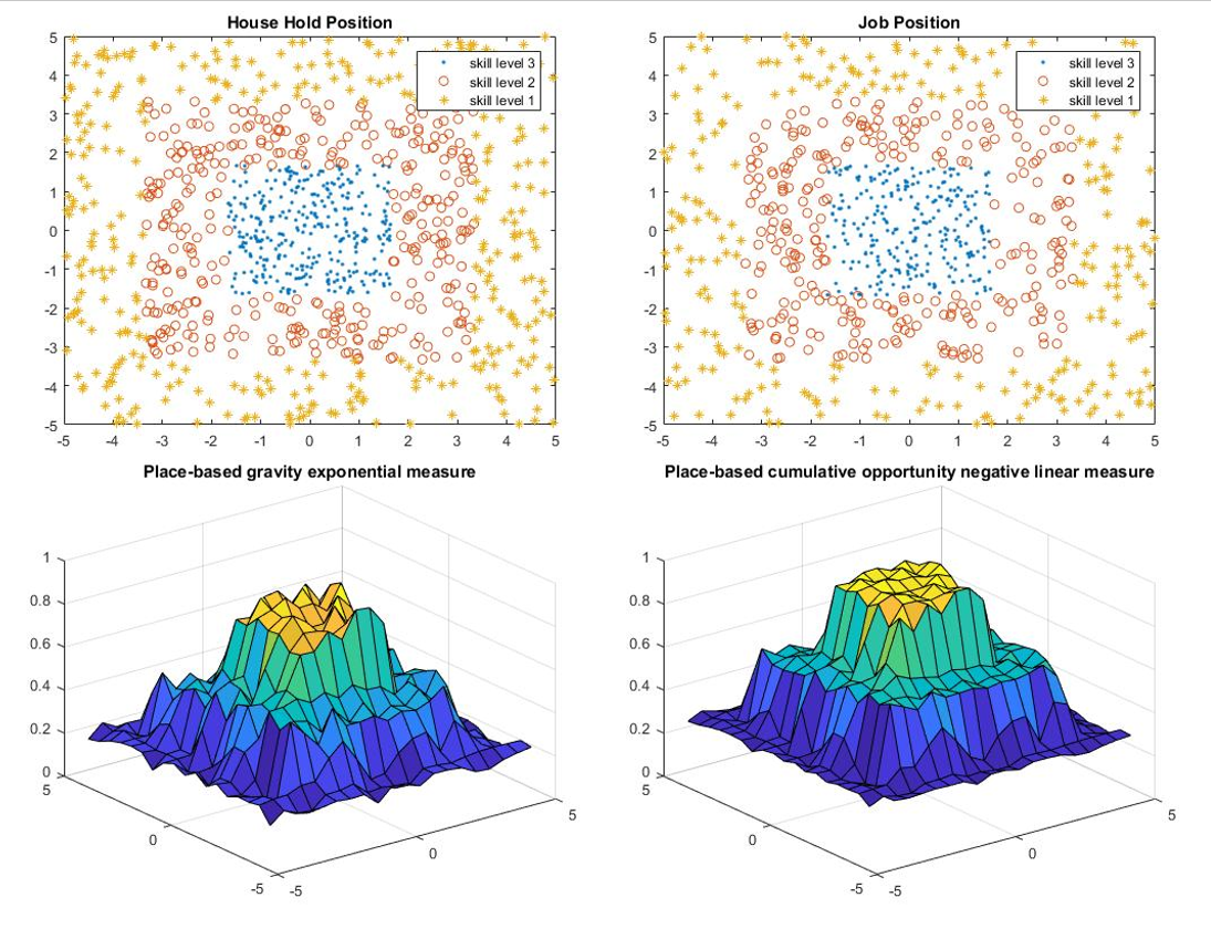
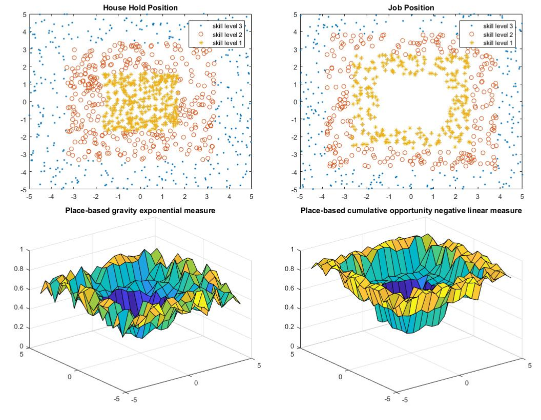
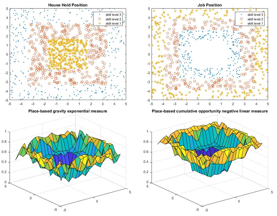
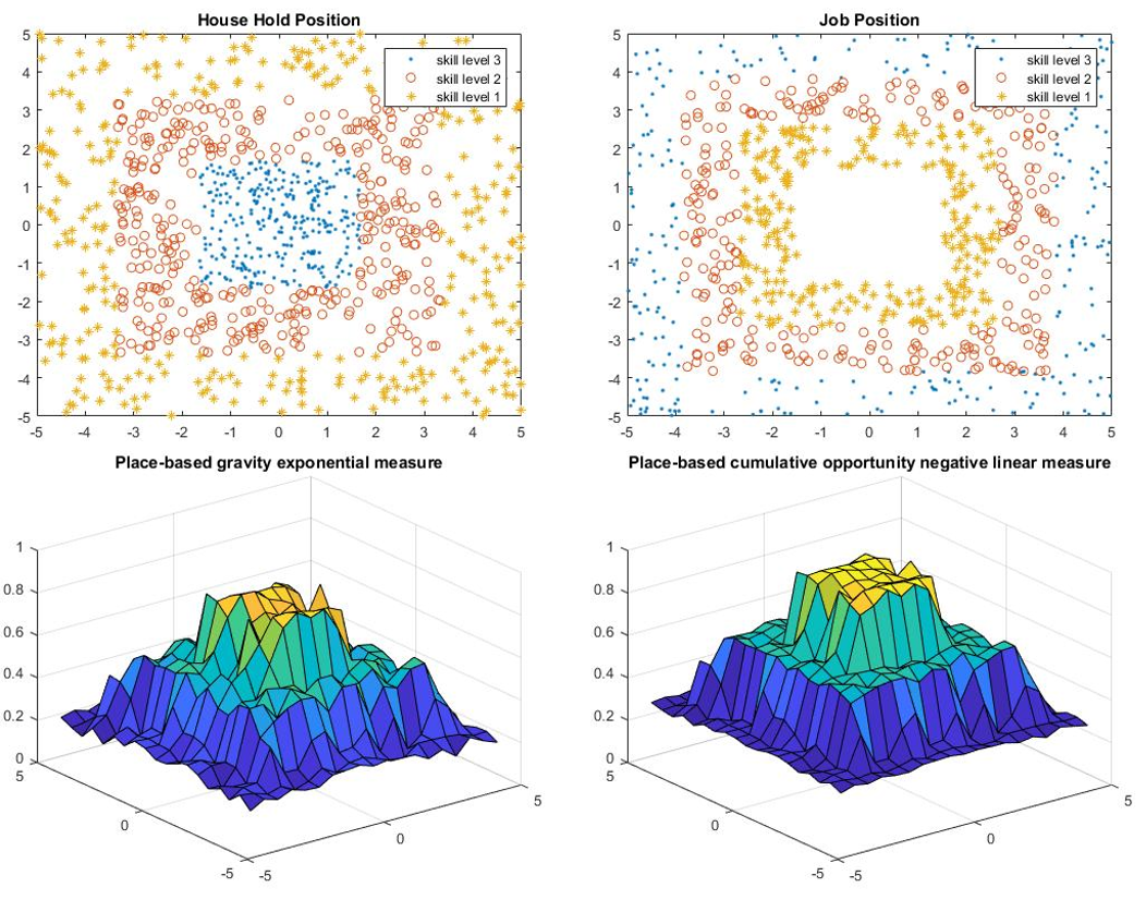
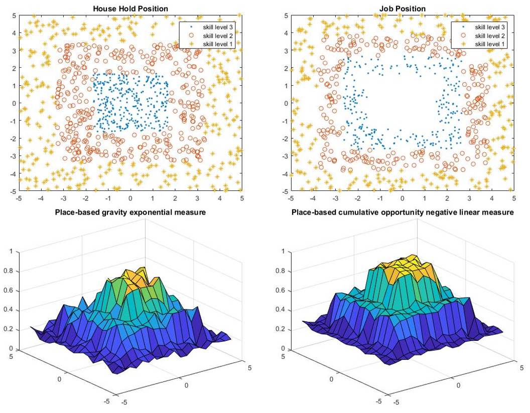
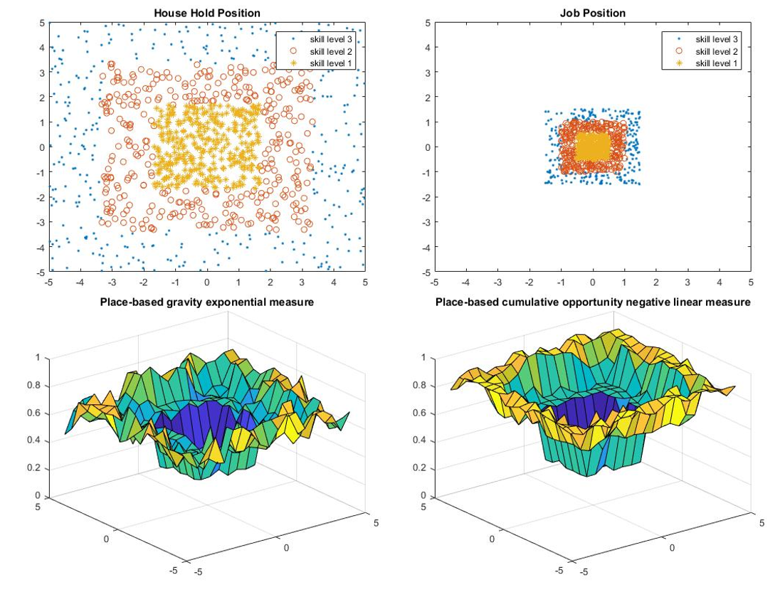
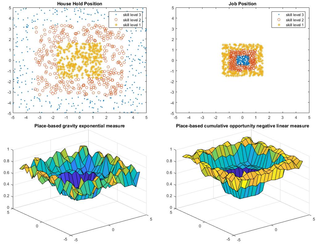
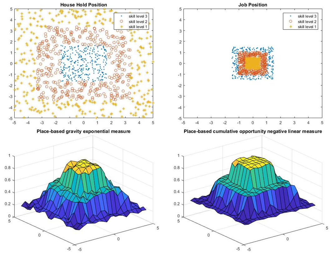
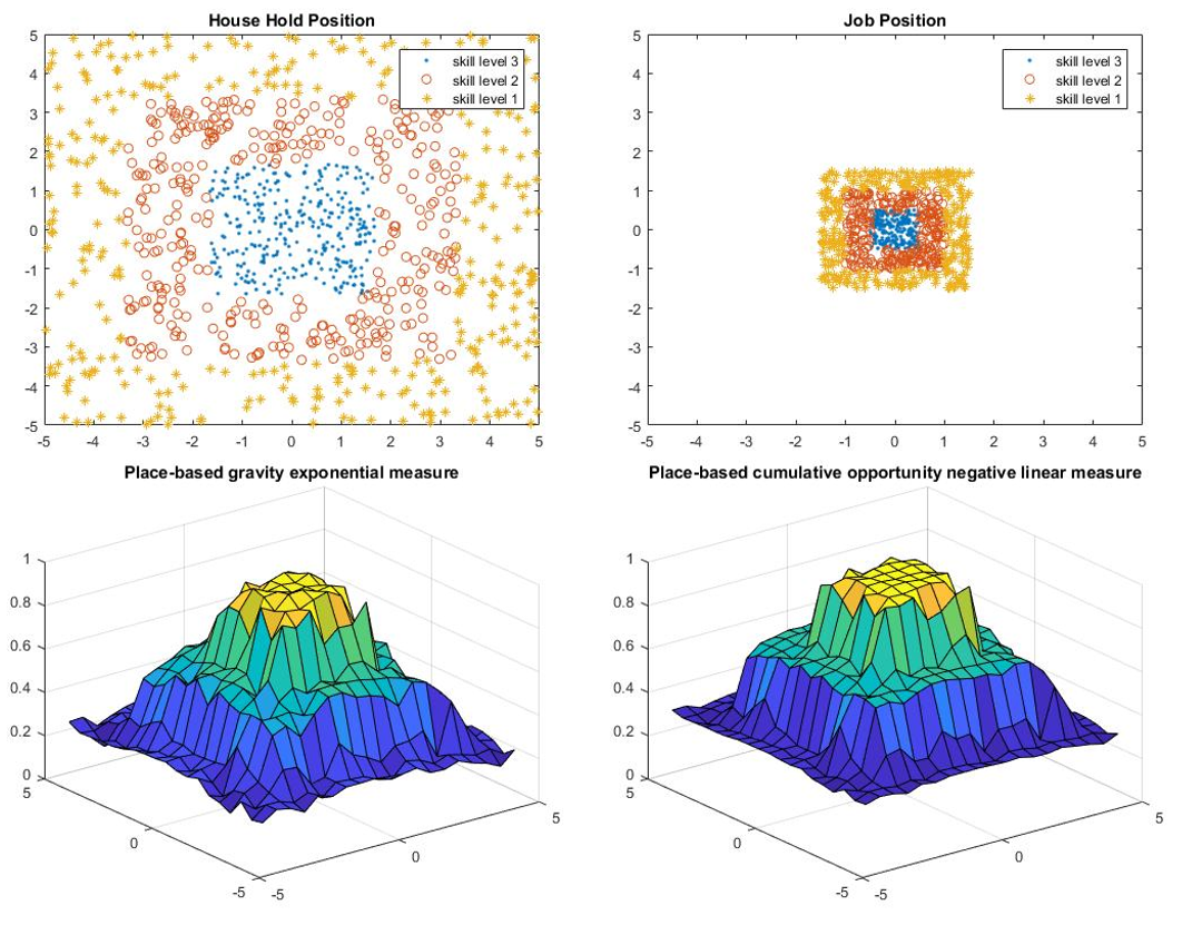
Household Location Relative to Job Location
Location comparison consists of four models: one upper bound, one lower bound, and two models in between.
- For upper bound, all people live in the center of the city and all jobs are located in the center of the city.
- For lower bound, all households and jobs are located in the periphery of the city.
- Model 1 refers to the model that has people living in the center and job located in the periphery, while model 2 refers to the opposite.
For all models, the number of people or household is 1000; the number of jobs are 800; the city is of size 10 by 10; the city center is of 3 by 3.
| Upper Bound | Lower Bound | Model 1 | Model 2 | |
|---|---|---|---|---|
| Gravity Measure | 0.9686 | 0.8888 | 0.9141 | 0.9136 |
| Percentage difference to lower bound | 8.97% | 0 | 2.85% | 2.79% |
| Cumulative Opportunity | 0.8958 | 0.6938 | 0.7460 | 0.7444 |
| Percentage difference to lower bound | 29.1% | 0 | 7.52% | 7.29% |
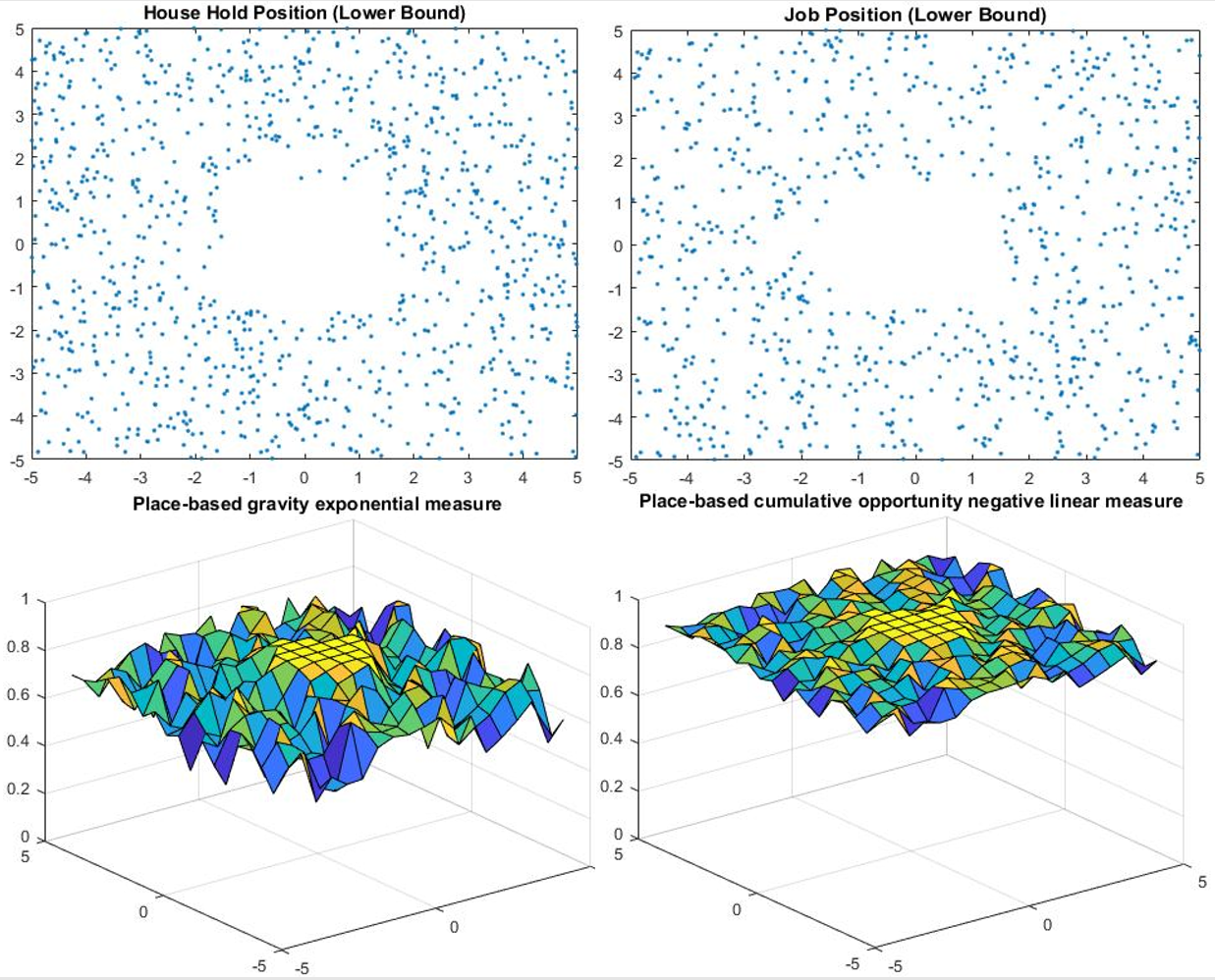
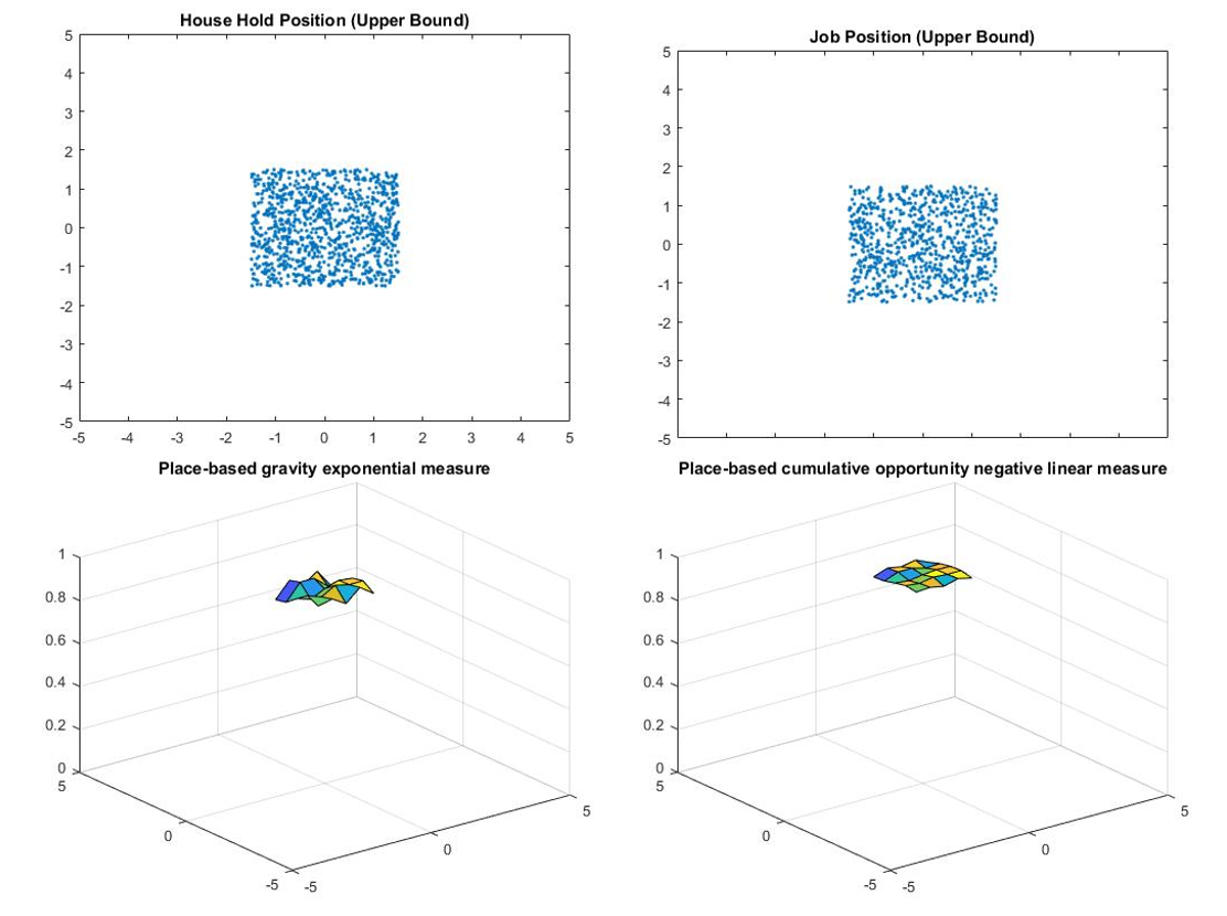
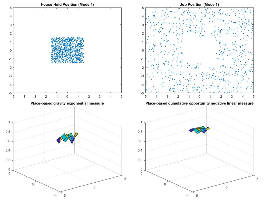
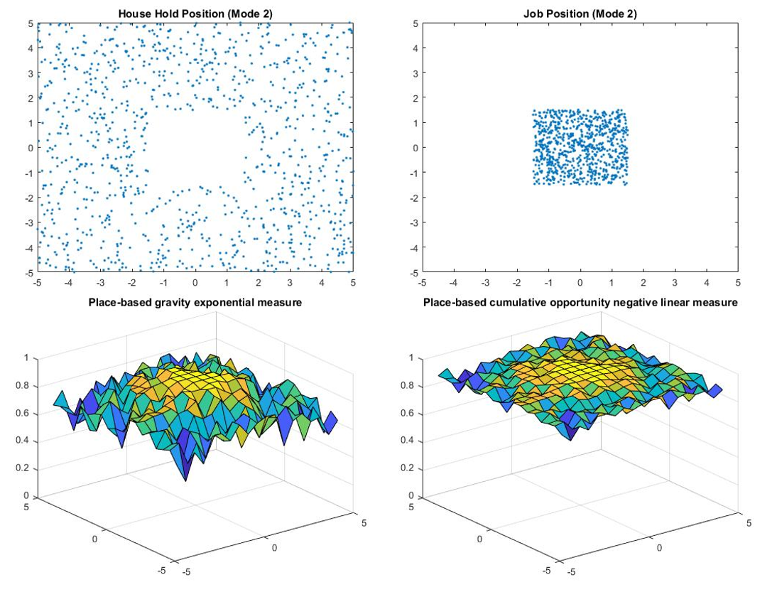
The results of the location comparison are presented in Table 1 and Figure 1-4.
Based on the results, the location may have a large effect on the accessibility as the percentage difference between upper bound and lower bound is large. However, the effects of changing the location of the household position and the job position are pretty similar because the percentage difference between model 1 and model 2 is small, and the difference may due to the total number of jobs is less than the total number of household positions.
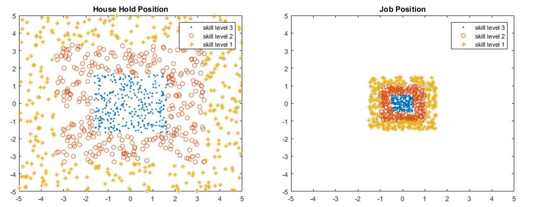
Job Density
For density comparisons, the model is set up with 1000 people with 3 skill levels and 800 jobs with 3 skill levels.
- The location of the people and jobs are assigned according to the skill levels.
- The people and jobs with higher skill levels will be closer to the center of the city.
- To investigate the influence of the job densities, the number of each skill level jobs is doubled separately.
People are only able to work on the job that has skill level lower or equal to his own skill level.
| Original Model | Double Skill Level 1 Job | Double Skill Level 2 Job | Double Skill Level 3 Job | |
|---|---|---|---|---|
| Gravity Measure | 0.4984 | 0.5812 | 0.5099 | 0.4070 |
| Percentage difference to original model | 0 | 16.6% | 2.3 | -18.3% |
| Cumulative Opportunity | 0.6023 | 0.7246 | 0.6077 | 0.4830 |
| Percentage difference to original model | 0 | 20.3% | 0.896% | -19.8% |
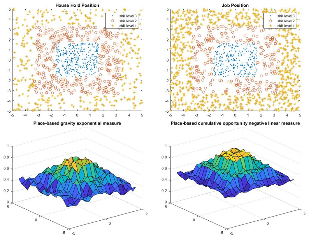
The results of the job density comparison are presented in Table 2 and Figure 5-8.
Based on the results, the lowest skill level density has a large influence on the overall accessibility, because everyone in the city is able to work on the lowest skill level jobs. The accessibility is not sensitive to the density of the medium level jobs. The density of the highest skill level job also has a large influence on the accessibility but in the opposite direction. That is because after doubling highest skill level jobs, the weight of the available job to lower skill level people decrease, which causes the drop of the overall accessibility.
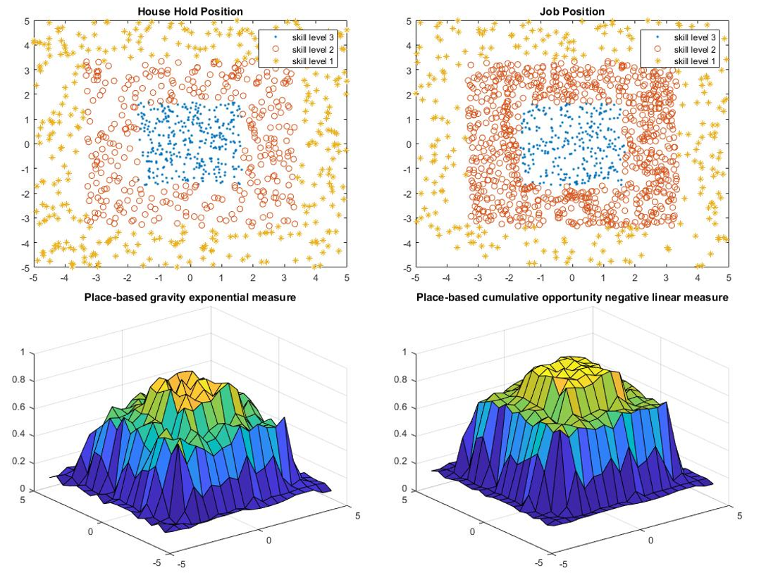
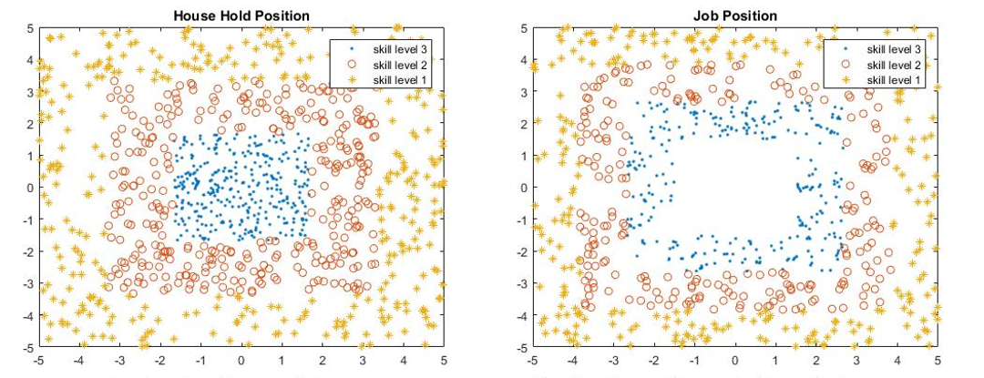
Skill Level Distribution
In skill level location comparisons, we further consider the city scale. People can live in any place in a city, but jobs are located in the periphery of a small city, while jobs in large city are located in the center of the city. Then the household position and job location are also distributed according to the skill level.
- Model 1 has both highest skill level people and jobs located in the periphery of the city, while the lowest skill level people and job located in the center.
- Model 2 keeps the location of people the same but switches the location of the highest skill level jobs and the lowest skill level jobs.
- Model 3 keeps the location of job the same with model 1 and switches the skill level location of people.
- Model 4 has both highest skill level people and job located in the center while the lowest located in the periphery.
| Small | City | Large | City | |||||
|---|---|---|---|---|---|---|---|---|
| Model 1 | Model 2 | Model 3 | Model 4 | Model 1 | Model 2 | Model 3 | Model 4 | |
| Gravity Measure | 0.4859 | 0.4775 | 0.4912 | 0.4708 | 0.5084 | 0.5302 | 0.5435 | 0.5686 |
| Percentage difference to model 1 | 0 | -1.73% | 1.10% | -3.11% | 0 | 4.29% | 6.90% | 11.8% |
| Cumulative Opportunity | 0.6013 | 0.6143 | 0.6011 | 0.5857 | 0.6096 | 0.6326 | 0.6183 | 0.6444 |
| Percentage difference to model 1 | 0 | 2.16% | -0.03% | -2.59% | 0 | 3.77% | 1.43% | 5.71% |
The results are shown in Table 3 and Figure 9-16.
For small city, the percentage difference has opposite signs of different measures. In that sense, we may regard the difference is due to random error, which means the skill level location does not have much influence on small cities. However, for large city, we can observe that model 1 has the lowest accessibility and model 4 has the highest accessibility. The distribution of skill level of model 4 is similar to that of real world large cities, which results in the largest accessibility in terms of skill level location.
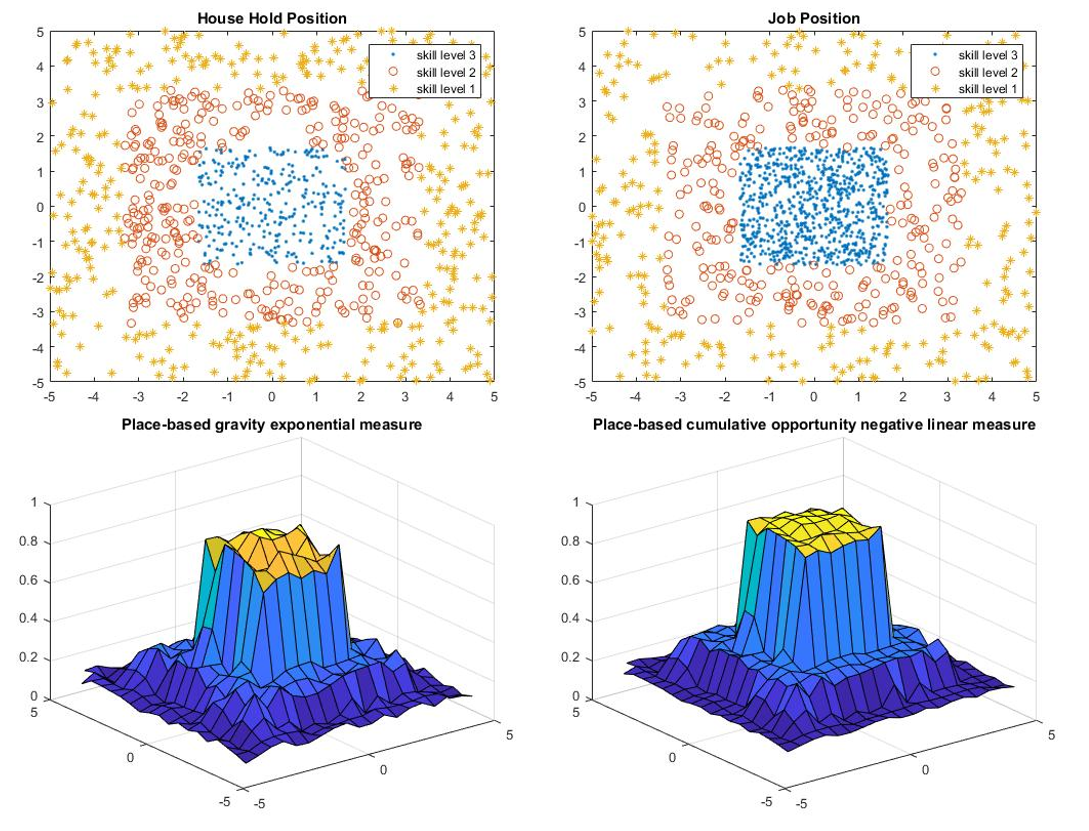
Transportation Method Change
For transportation change, we again consider the city scale. The household location and job location of large cities and small cities are shown in Figure 17 and Figure 18 respectively. We consider four models for transportation change.
- In model 1, everyone in the city drive to work (upper bound),
- while in model 2, everyone walk to work (lower bound).
- In model 3, people with skill level 3 drive to work; people with skill level 2 take bus; and people with skill level 1 walk.
- Model 4 is similar to model 3, and the only difference is skill level 2 people drive or take bus to work.
| Small | City | Large | City | |||||
|---|---|---|---|---|---|---|---|---|
| Model 1 | Model 2 | Model 3 | Model 4 | Model 1 | Model 2 | Model 3 | Model 4 | |
| Gravity Measure | 0.5523 | 0.3907 | 0.5184 | 0.4879 | 0.5962 | 0.5009 | 0.5446 | 0.5484 |
| Percentage difference to model 2 | 41.4% | 0 | 32.7% | 24.9% | 19.0% | 0 | 8.72% | 9.48% |
| Cumulative Opportunity | 0.6289 | 0.5569 | 0.6247 | 0.5966 | 0.6408 | 0.6157 | 0.6157 | 0.6157 |
| Percentage difference to model 2 | 12.9/% | 0 | 12.3% | 7.13% | 4.08% | 0 | 0.16% | 1.17% |
The results are shown in Table 4 and Figure 19-26.
Note that for different models, the accessibility measure has the similar shape, and only the magnitude changes. Generally, transportation mode has a large influence on the accessibility. The influence is especially obvious in small city. Since the travel distance for skill level 2 people is relatively small in large city, there will not be much difference between driving or taking bus, so the accessibilities of model 3 and model 4 are similar to each other.